Richard M. Ennis

Mar 17, 2022 by Richard M. Ennis

Alternative investments and novel strategies, such as risk parity and smart beta, have brought about a blurring of the asset allocation profile of many institutional investors. In days gone by, the funds described their holdings in terms of U.S. stocks, non-U.S. stocks, investment-grade bonds, and, maybe, high-quality unlevered properties (real estate).  The vocabulary of institutional investors is very different now. For one thing, the funds define asset classes however they see fit. Ambiguous descriptions include “real assets,” “risk mitigation,” “opportunistic,” “risk parity,” “diversifying,” “multi-risk,” “alternative beta,” “absolute return,” “alpha pool,” “alternative” and, my favorite, “unique.” Some asset types are hybrid: hedge funds, for example, behave like a blend of equity and fixed income securities, and it would be a mistake to classify them as one or the other. Some fixed income assets, such as junk bonds, or anything with “credit” in the name, may be as equity-like as bond-like. Going by asset class labels, it is difficult to know what to make of modern day institutional portfolios in terms their market exposures. 

 

            I estimate the effective exposure of institutional funds to major markets using the multiple regression method developed by William Sharpe.[1] Commonly known as returns-based style analysis (RBSA), the technique allows one to infer market exposures from the returns generated by a portfolio or a composite of them. In using RBSA to identify the market exposure of public pension funds in the U.S., I regress the returns of a composite of 46 public funds for the 13 years ended June 30, 2021, against independent variables for Russell 3000 stocks, MSCI All-Country World ex-U.S. stocks (unhedged and hedged), and Bloomberg U.S. Aggregate bonds. The betas that result from the multiple regression indicate the effective percentage exposure to each index. Application of RBSA establishes the market exposure of the composite as follows: 55% U.S. equity, 17% non-U.S. equity, and 28% bonds.[2] This means that, over time, the returns of the composite have resembled those of a benchmark comprising these indexes in these proportions. And by this means we altogether bypass asset class labels in favor of a parsimonious expression of major market exposures. How effective is RBSA in establishing a useful market-based profile?

 

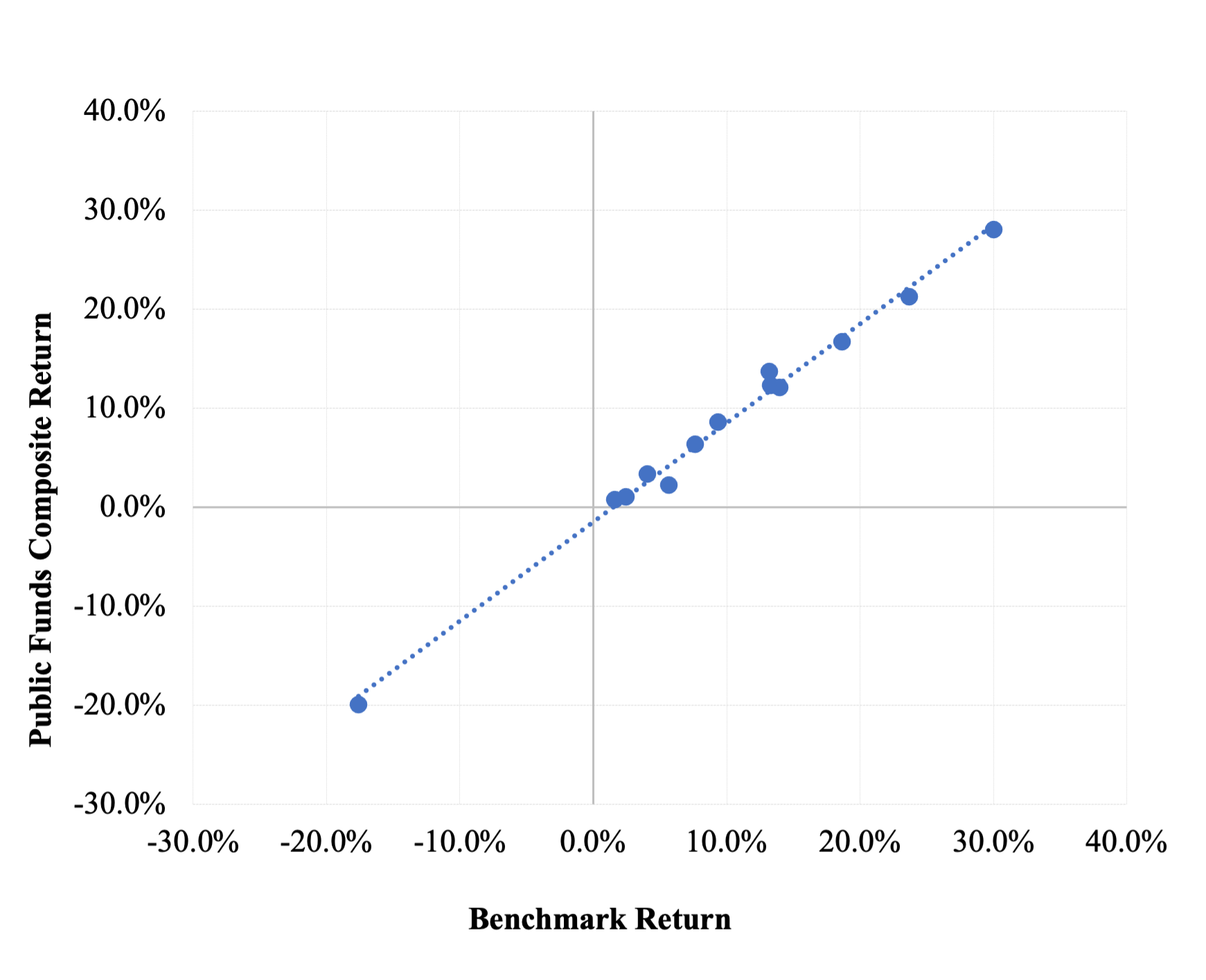
            Exhibit 1 illustrates the regression of the public fund composite on a benchmark comprising the market weights described above. The benchmark’s three broad market components explain an eye-popping 99.2% (R²) of the annual variation in return of public funds in aggregate. (I made no attempt to “unsmooth” the returns of alternative investments, which account for 32% of the composite’s assets, according to Cliffwater LLC.) Annualized tracking error is just 1.0%. The power of the model derives from two facts: (1) public pension funds diversify their holdings extensively, and (2) the funds maintain a fairly stable asset allocation over time. RBSA embodies an age-old, pragmatic worldview: If something walks, quacks and swims like a duck, it can reasonably be cast as a duck.

 

 

Exhibit 1

Regression of Composite on Benchmark

13 Years Ended June 30, 2021
 

             An important implication of this analysis is that adding alternative investments has not had a material impact on public funds’ diversification beyond that which can be obtained by simply combining stock and bond index funds. These results run counter to the notion that the return properties of alts differ materially from those of stocks and bonds. That, after all, is an oft-cited reason for incorporating alternative investments in the portfolio along with stocks and bonds. But as we see here, alt returns simply blend in with broad market returns, and those of U.S. markets, in particular, in the context of standard portfolio analysis.     

 

            The prominence of the Russell 3000 index in the analysis comes as no real surprise when we take account of the high degree of correlation between principal alternative investment categories and the U.S. equity market. Exhibit 2 shows the correlation coefficients for three of the main areas of alternative investment with the Russell 3000 stock index; the average value is .93. Hence, the lion’s share of the alts reported as accounting for nearly a third of public fund assets is strongly statistically associated with the U.S.-stock-market variable in an analysis like this.

 

 

Exhibit 2

Alts’ Correlation with U.S. Equities

Twelve Years Ended June 30, 2020

Alternative Asset  Category	Correlation Coefficient
Buyouts	.98
Real Estate	.88
Hedge Funds	.94
Average	.93

Sources: Cambridge Associates 

(for buyouts and real estate), HFR

 

            Exhibit 3 illustrates the power of RBSA as an analytical tool at the individual fund level. Shown there are each of the funds that make up the composite described above. The analysis uses the same market indexes as described above. Effective equity exposures range from a low of 58% to a high of 87%. The R²s are very high at all levels of equity exposure. The median is .987, and just three values fall below .950. The high R²s of the individual funds underscore the degree of diversification that is characteristic of public funds. Those same statistics also indicate the explanatory power of RBSA, even as applied at the individual fund level.

 

Exhibit 3

Individual Fund Analysis

Twelve Years Ended June 30, 2020

 

Rank	Fund	Effective Equity Exposure	R2	Alpha	t-Stat
1	West Virginia PERS	70%	0.987	1.56%	3.75
2	Arkansas Teachers	79	0.963	0.91	1.19
3	Georgia Teachers	62	0.992	0.90	3.00
4	Arizona SRS	73	0.985	0.39	0.81
5	New Jersey	66	0.977	0.26	0.48
6	Minnesota SBI	76	0.995	0.23	0.77
7	Connecticut Teachers	68	0.993	0.14	0.47
8	Los Angeles DWP	67	0.996	0.07	0.32
9	Kentucky County	68	0.974	-0.09	-0.16
10	New Hampshire	74	0.989	-0.34	-0.79
11	New York City ERS	70	0.995	-0.34	-1.18
12	Connecticut Employees	70	0.992	-0.34	-1.05
13	Florida	74	0.996	-0.43	-1.64
14	North Carolina	58	0.996	-0.51	-2.45
15	South Dakota	83	0.967	-0.63	-0.75
16	New Mexico Teachers	67	0.925	-0.66	-0.62
17	Illinois Universities	73	0.992	-0.86	-2.25
18	Iowa PERS	63	0.984	-0.88	-1.86
19	Maine	70	0.987	-0.93	-2.08
20	Los Angeles County	71	0.992	-1.05	-2.99
21	Arizona Pub Safety	68	0.978	-1.56	-2.92
22	San Francisco	79	0.987	-1.66	-3.31
23	South Carolina	69	0.962	-1.67	-2.23
24	New York State Teachers	76	0.996	-1.71	-5.89
25	Washington State	77	0.982	-1.87	-3.12
26	Rhode Island	69	0.992	-1.89	-5.27
27	Illinois State Employees	77	0.991	-1.92	-4.92
28	Ohio School Employees	78	0.994	-2.03	-6.24
29	Montana	75	0.993	-2.10	-5.65
30	Virginia Ret. System	73	0.978	-2.21	-3.55
31	Texas Teachers	75	0.970	-2.24	-2.93
32	Oregon	78	0.968	-2.29	-2.80
33	Vermont Teachers	66	0.949	-2.37	-2.52
34	Phoenix ERS	72	0.993	-2.37	-6.81
35	Illinois Teachers Ret Sys	80	0.991	-2.52	-5.81
36	Maryland State Ret	69	0.984	-2.57	-4.99
37	California STRS	83	0.994	-2.63	-7.08
38	Missouri DOT & HP	81	0.972	-2.72	-3.52
39	North Dakota ERS	82	0.991	-2.82	-6.49
40	New Mexico PERA	80	0.973	-3.09	-4.03
41	Kern County	73	0.988	-3.13	-6.65
42	California PERS	79	0.991	-3.13	-7.26
43	Indiana PERS	66	0.947	-3.42	-3.60
44	North Dakota Teachers	87	0.989	-3.70	-6.89
45	Missouri SERS	67	0.929	-3.81	-3.22
46	Pennsylvania Pub Sch	75	0.951	-3.91	-3.80
	Median	73%	0.987	-1.69%	n/a

 

            RBSA does more than provide a framework for understanding and comparing market exposures and risk characteristics. It offers a theoretically sound way to evaluate performance. By comparing a fund’s (or composite’s) return to that of its RBSA benchmark, we can determine the value-added relative to a passively investable benchmark. For example, the regression analysis for the composite depicted in Exhibit 1 has an intercept (alpha) of -1.45% per year. The t-stat of the alpha is -4.0, indicating a margin of underperformance that is both economically large and statistically significant. Exhibit 3 shows the alpha and t-stat for the individual funds making up the composite. Thirty of 46 funds (65%) have negative alphas that are statistically significant. Only two funds have positive alphas that are statistically significant. The poor performance is a consequence of extreme diversification of individual funds combined with a typical investment cost of 1.3% of asset value.[3]

 

            Summing up: We need not be baffled by ambiguous asset-class labels. We have tools like RBSA to help us decipher institutional investors’ market exposures and risk characteristics, and evaluate their performance. The funds could give their asset categories labels like “third base,” “Carlos,” and “serendipity,” but that wouldn’t keep us from gleaning important insights about their investment character and performance. The information we need is embedded in the return history.

 

REFERENCES

 

Ennis, R. M. 2022. “Cost, Performance, and Benchmark Bias of Public Pension Funds in the United States: An Unflattering Portrait.” Forthcoming, Journal of Portfolio Management. Currently available at https://papers.ssrn.com/sol3/papers.cfm?abstract_id=3883370

Prev Next